Probability plots to check the goodness of fit of parametric models

probPlot provides four types of probability plots: P-P plot, Q-Q plot, Stabilised probability plot, and Empirically Rescaled plot to check if a certain distribution is an appropiate choice for the data.

# Default S3 method
probPlot(times, cens = rep(1, length(times)),
         distr = c("exponential", "gumbel", "weibull", "normal",
                   "lognormal", "logistic", "loglogistic", "beta"),
         plots = c("PP", "QQ", "SP", "ER"),
         colour = c("green4", "deepskyblue4", "yellow3",
                    "mediumvioletred"), mtitle = TRUE, ggp = FALSE,
         m = NULL, betaLimits = c(0, 1), igumb = c(10, 10),
         prnt = TRUE, degs = 3,
         params0 = list(shape = NULL, shape2 = NULL,
                        location = NULL, scale = NULL), print.AIC = TRUE,
                        print.BIC = TRUE, ...)
# S3 method for class 'formula'
probPlot(formula, data, ...)

Arguments

times: Numeric vector of times until the event of interest.
cens: Status indicator (1, exact time; 0, right-censored time). If not provided, all times are assumed to be exact.
distr: A string specifying the name of the distribution to be studied. The possible distributions are the exponential ("exponential"), the Weibull ("weibull"), the Gumbel ("gumbel"), the normal ("normal"), the lognormal ("lognormal"), the logistic ("logistic"), the loglogistic ("loglogistic"), and the beta ("beta") distribution.
plots: Vector stating the plots to be displayed. Possible choices are the P-P plot ("PP"), the Q-Q plot ("QQ"), the Stabilised Probability plot ("SP"), and the Empirically Rescaled plot ("ER"). By default, all four plots are displayed.
colour: Vector indicating the colours of the displayed plots. The vector will be recycled if its length is smaller than the number of plots to be displayed.
mtitle: Logical to add or not the title "Probability plots for a distr distribution" to the plot. Default is TRUE.
ggp: Logical to use or not the ggplot2 package to draw the plots. Default is FALSE.
m: Optional layout for the plots to be displayed.
betaLimits: Two-components vector with the lower and upper bounds of the Beta distribution. This argument is only required, if the beta distribution is considered.
igumb: Two-components vector with the initial values for the estimation of the Gumbel distribution parameters.
prnt: Logical to indicate if the maximum likelihood estimates of the parameters should be printed. Default is TRUE.
degs: Integer indicating the number of decimal places of the numeric results of the output.
params0: List specifying the parameters of the theoretical distribution. By default, parameters are set to NULL and estimated with the maximum likelihood method. This argument is only considered, if all parameters of the studied distribution are specified.
formula: A formula with a numeric vector as response (which assumes no censoring) or Surv object.
data: Data frame for variables in formula.
print.AIC: Logical to indicate if the AIC of the model should be printed. Default is TRUE
print.BIC: Logical to indicate if the BIC of the model should be printed. Default is TRUE
...: Optional arguments for function par, if ggp = FALSE.

Details

By default, function probPlot draws four plots: P-P plot, SP plot, Q-Q plot, and EP plot. Following, a description is given for each plot.

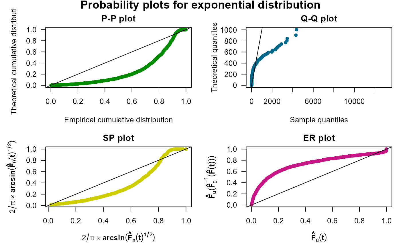
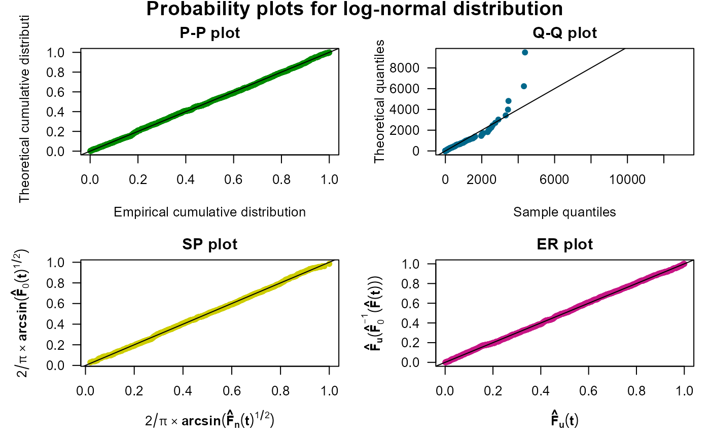
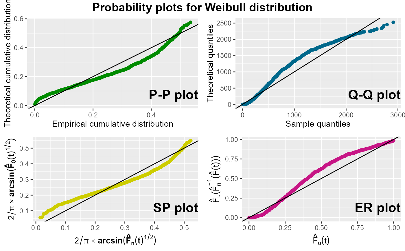
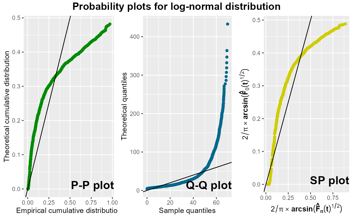
The Probability-Probability plot (P-P plot) depicts the empirical distribution, \(\widehat{F}(t)\), which is obtained with the Kaplan-Meier estimator if data are right-censored, versus the theoretical cumulative distribution function (cdf), \(\widehat{F_0}(t)\). If the data come from the chosen distribution, the points of the resulting graph are expected to lie on the identity line.

The Stabilised Probability plot (SP plot), proposed by Michael (1983), is a transformation of the P-P plot. It stabilises the variance of the plotted points. If \(F_0 = F\) and the parameters of \(F_0\) are known, \(\widehat{F_0}(t)\) corresponds to the cdf of a uniform order statistic, and the arcsin transformation stabilises its variance. If the data come from distribution \(F_0\), the SP plot will resemble the identity line.

The Quartile-Quartile plot (Q-Q plot) is similar to the P-P plot, but it represents the sample quantiles versus the theoretical ones, that is, it plots \(t\) versus \(\widehat{F}_0^{-1}(\widehat{F}(t))\). Hence, if \(F_0\) fits the data well, the resulting plot will resemble the identity line.

A drawback of the Q-Q plot is that the plotted points are not evenly spread. Waller and Turnbull (1992) proposed the Empirically Rescaled plot (EP plot), which plots \(\widehat{F}_u(t)\) against \(\widehat{F}_u(\widehat{F}_0^{-1}(\widehat{F}(t)))\), where \(\widehat{F}_u(t)\) is the empirical cdf of the points corresponding to the uncensored observations. Again, if \(\widehat{F}_0\) fits the data well, the ER plot will resemble the identity line.

By default, all four probability plots are drawn and the maximum likelihood estimates of the parameters of the chosen parametric model are returned. The parameter estimation is acomplished with the fitdistcens function of the fitdistrplus package.

Value

If prnt = TRUE, the following output is returned:

Distribution: Distribution under study.
Parameters: Parameters used to draw the plots (if params0 is provided).
Estimates: A list with the maximum likelihood estimates of the parameters of all distributions considered.
StdErrors: Vector containing the estimated standard errors.
aic: The Akaike information criterion.
bic: The so-called BIC or SBC (Schwarz Bayesian criterion).

In addition, a list with the same contents is returned invisibly.

References

J. R. Michael. The Stabilized Probability Plot. In: Biometrika 70 (1) (1983), 11-17.

L.A. Waller and B.W. Turnbull. Probability Plotting with Censored Data. In: American Statistician 46 (1) (1992), 5-12.

Author

K. Langohr, M. Besalú, M. Francisco, A. Garcia, G. Gómez.

Examples

# P-P, Q-Q, SP, and EP plots for complete data
set.seed(123)
x <- rlnorm(1000, 3, 2)
probPlot(x)
#> Distribution: exponential 
#>   
#> Parameter estimates:
#>    Scale (se): 145.449 (4.599)
#> 
#>    AIC: 11961.65 
#>    BIC: 11966.55 
#> 

probPlot(x, distr = "lognormal")
#> Distribution: log-normal 
#>   
#> Parameter estimates:
#> Location (se): 3.032 (0.063)
#>    Scale (se): 1.982 (0.044)
#> 
#>    AIC: 10275 
#>    BIC: 10284.82 
#> 


# P-P, Q-Q, SP, and EP plots for censored data using ggplot2
probPlot(Surv(time, status) ~ 1, colon, "weibull", ggp = TRUE)
#> Distribution: Weibull 
#>   
#> Parameter estimates:
#>    Shape (se): 0.796 (0.024)
#>    Scale (se): 3529.763 (163.053)
#> 
#>    AIC: 16575.45 
#>    BIC: 16586.51 
#> 


# P-P, Q-Q and SP plots for censored data and lognormal distribution
data(nba)
probPlot(Surv(survtime, cens) ~ 1, nba, "lognorm", plots = c("PP", "QQ", "SP"),
         ggp = TRUE, m = matrix(1:3, nr = 1))
#> Distribution: log-normal 
#>   
#> Parameter estimates:
#> Location (se): 4.287 (0.029)
#>    Scale (se): 0.942 (0.021)
#> 
#>    AIC: 9917.451 
#>    BIC: 9930.02 
#>