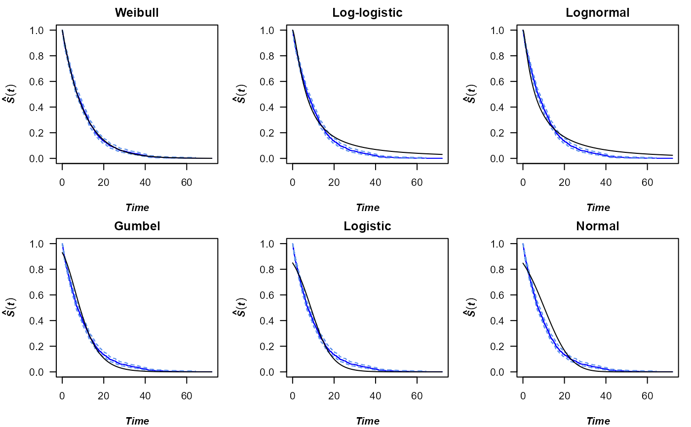
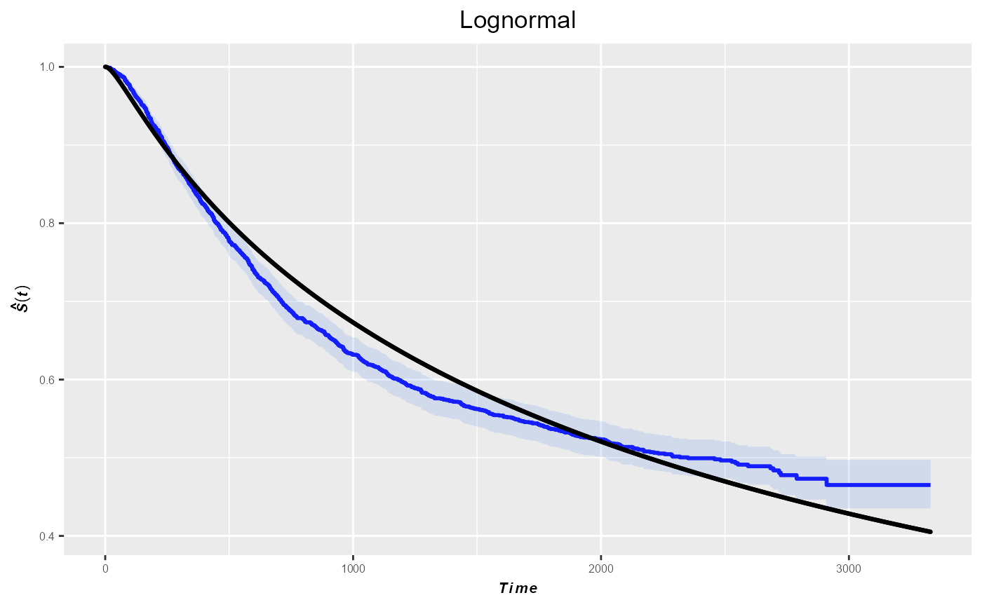
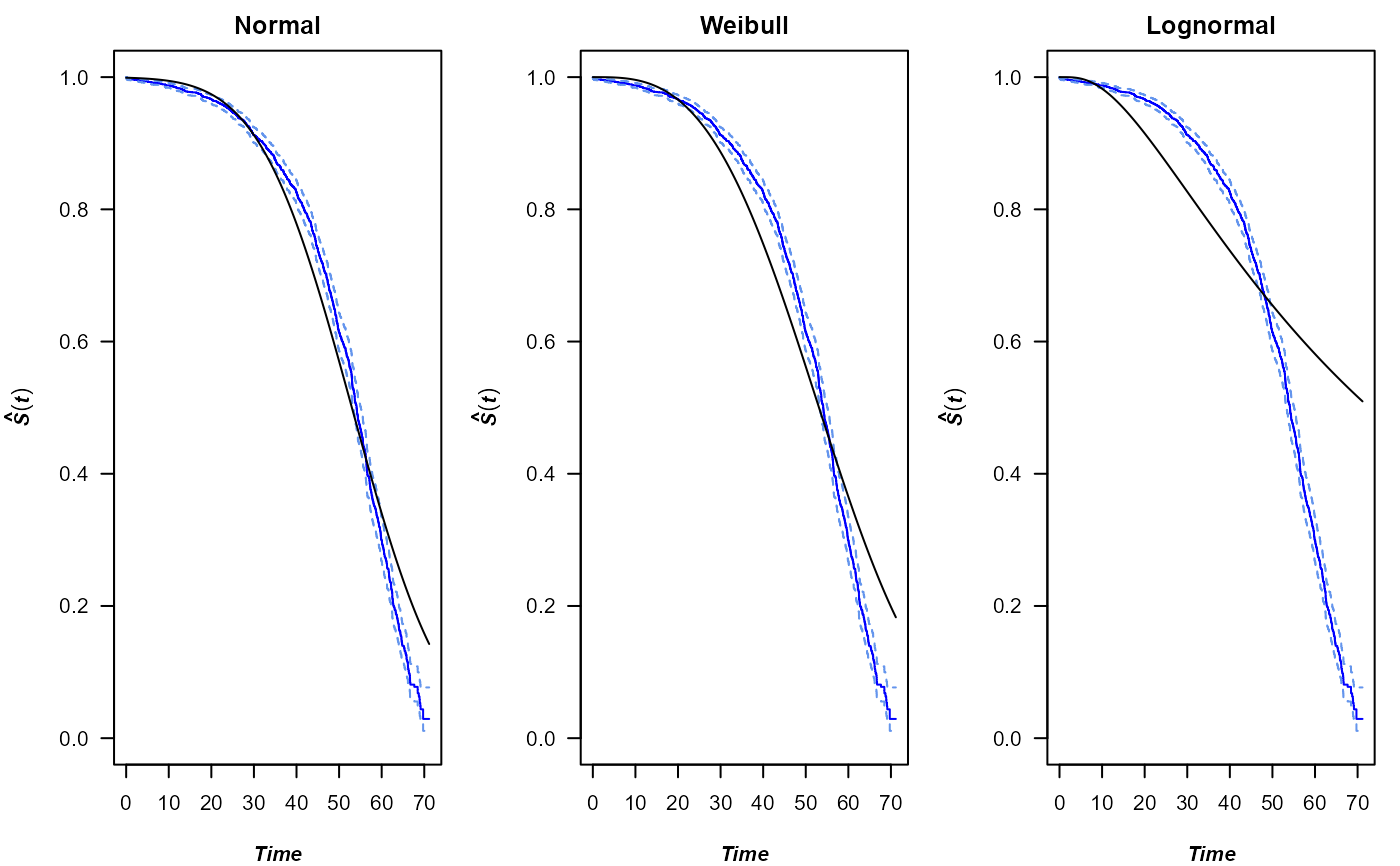
Plot of the Kaplan-Meier and parametric estimations

Function kmPlot is a function that generates a plot that combines a Kaplan-Meier survival curve and a parametric survival curve in the same graph. It is useful for comparing non-parametric survival estimates with the fitted parametric survival model.

# Default S3 method
kmPlot(times, cens = rep(1, length(times)), distr = "all6",
       colour = c("black", "blue", "cornflowerblue"),
       betaLimits = c(0, 1), igumb = c(10, 10), ggp = FALSE, m = NULL,
       prnt = TRUE, degs = 3, print.AIC = TRUE, print.BIC = TRUE,...)
# S3 method for class 'formula'
kmPlot(formula, data, ...)

Arguments

times: Numeric vector of times until the event of interest.
cens: Status indicator (1, exact time; 0, right-censored time). If not provided, all times are assumed to be exact.
distr: A string specifying the name of the distribution to be studied. The possible distributions are the Weibull ("weibull"), the Gumbel ("gumbel"), the normal ("normal"), the lognormal ("lognormal"), the logistic ("logistic"), the loglogistic ("loglogistic"), the exponential ("exponential") and the beta ("beta") distribution. Default is "all6" and includes the fisrt 6 listed which are the most used distributions.
colour: Vector with three components indicating the colours of the displayed plots. The first element is for the survival curve, the second for the Kaplan-Meier curve, and the last one for the confidence intervals.
betaLimits: Two-components vector with the lower and upper bounds of the Beta distribution. This argument is only required, if the beta distribution is considered.
igumb: Two-components vector with the initial values for the estimation of the Gumbel distribution parameters.
ggp: Logical to use or not the ggplot2 package to draw the plots. Default is FALSE.
m: Optional layout for the plots to be displayed.
prnt: Logical to indicate if the maximum likelihood estimates of the parameters should be printed. Default is TRUE.
degs: Integer indicating the number of decimal places of the numeric results of the output.
formula: A formula with a numeric vector as response (which assumes no censoring) or Surv object.
data: Data frame for variables in formula.
print.AIC: Logical to indicate if the AIC of the model should be printed. Default is TRUE
print.BIC: Logical to indicate if the BIC of the model should be printed. Default is TRUE
...: Optional arguments for function par, if ggp = FALSE.

Details

The parameter estimation is acomplished with the fitdistcens function of the fitdistrplus package.

Value

If prnt = TRUE, the following output is returned:

Distribution: Distribution under study.
Estimates: A list with the maximum likelihood estimates of the parameters of all distributions considered.
StdErrors: Vector containing the estimated standard errors.
aic: The Akaike information criterion.
bic: The so-called BIC or SBC (Schwarz Bayesian criterion).

In addition, a list with the same contents is returned invisibly.

References

Peterson Jr, Arthur V. Expressing the Kaplan-Meier estimator as a function of empirical subsurvival functions. In: Journal of the American Statistical Association 72.360a (1977): 854-858.

Author

K. Langohr, M. Besalú, M. Francisco, A. Garcia, G. Gómez.

Examples

# Plots for complete data and default distributions
set.seed(123)
x <- rexp(1000, 0.1)
kmPlot(x)
#> Parameter estimates
#>   
#> weibull
#>    Shape (se): 1.014 (0.025)
#>    Scale (se): 10.359 (0.34)
#>    AIC: 6667.949 
#>    BIC: 6677.764 
#> 
#> loglogistic
#>    Shape (se): 1.441 (0.038)
#>    Scale (se): 6.597 (0.251)
#>    AIC: 6808.804 
#>    BIC: 6818.619 
#> 
#> lognormal
#> Location (se): 1.764 (0.04)
#>    Scale (se): 1.275 (0.029)
#>    AIC: 6856.968 
#>    BIC: 6866.784 
#> 
#> gumbel
#> Location (se): 6.184 (0.209)
#>    Scale (se): 6.332 (0.169)
#>    AIC: 6994.971 
#>    BIC: 7004.786 
#> 
#> logistic
#> Location (se): 8.798 (0.275)
#>    Scale (se): 5.076 (0.136)
#>    AIC: 7307.124 
#>    BIC: 7316.94 
#> 
#> normal
#> Location (se): 10.3 (0.317)
#>    Scale (se): 10.039 (0.224)
#>    AIC: 7454.836 
#>    BIC: 7464.652 
#> 


# Plots for censored data using ggplot2
kmPlot(Surv(time, status) ~ 1, colon, distr= "lognormal", ggp = TRUE)
#> Parameter estimates
#>   
#> lognormal
#> Location (se): 7.691 (0.05)
#>    Scale (se): 1.748 (0.046)
#>    AIC: 16445.98 
#>    BIC: 16457.04 
#> 


# Plots for censored data from three distributions
data(nba)
kmPlot(Surv(survtime, cens) ~ 1, nba, distr = c("normal", "weibull", "lognormal"),
       prnt = FALSE)